Running Analyses

This guide walks through running a transient simulation — using a low-pass filter as a worked example. You'll set up an AC signal source, place probes to capture node voltages, configure a transient analysis, and read the results.

Step 1 — Add an AC source in series with the DC supply

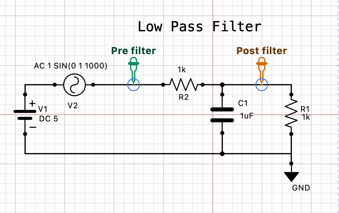
To simulate a signal riding on a DC bias, place an AC voltage source (V2) in series with your DC supply (V1). The AC source provides the time-varying stimulus while the DC source sets the operating point.

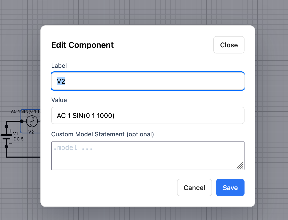
Double-click the AC source to open the component editor and set its value to:

AC 1 SIN(0 1 1000)

This tells ngspice the source is an AC source with amplitude 1, and a sinusoidal waveform at 1 kHz with zero DC offset and 1 V peak.

Component editor showing V2 with value AC 1 SIN(0 1 1000)

Step 2 — Place probes

Press P or click the Probe tool in the toolbar to enter probe mode. Click any wire or node to place a voltage probe at that point. Each probe is auto-labelled and will appear as a separate trace in the results panel.

For this filter example, two probes were placed:

Pre filter — on the node between V2 and the resistor R2, capturing the unfiltered signal.
Post filter — on the output node after the RC network, capturing the filtered signal.

Low-pass filter schematic with Pre filter and Post filter probes placed

Step 3 — Configure a transient analysis

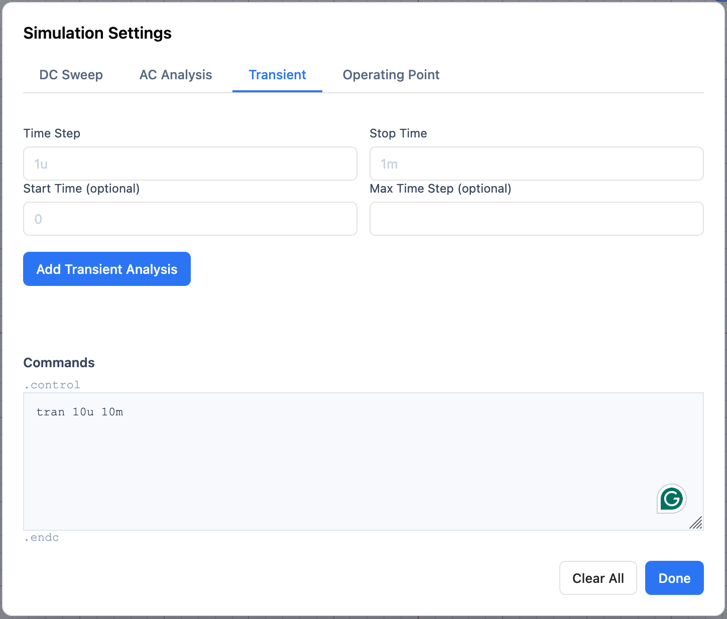
Open the Simulation Settings panel by clicking the settings icon in the Results panel header. Select the Transient tab.

Set the simulation parameters:

Time Step — the maximum time step ngspice will use internally (e.g. 10u for 10 µs).
Stop Time — how long to simulate (e.g. 10m for 10 ms, giving 10 full cycles at 1 kHz).

Click Add Transient Analysis to add it to the command list. The generated ngspice command appears in the Commands box:

tran 10u 10m

Click Done to close the settings panel.

Simulation Settings panel with Transient tab showing tran 10u 10m

Step 4 — Run and read the results

Click the green Run button (▶) at the top of the Results panel. SpicePad sends the netlist to the ngspice WebAssembly engine and streams back the results.

Once complete, a "Simulation complete" banner appears and the transient plot is displayed below it. Each probe trace is colour-coded and labelled in the legend.

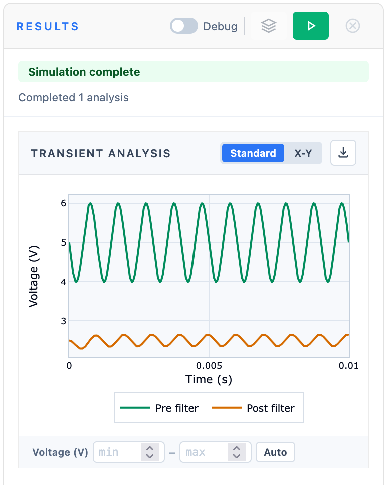
Results panel showing transient analysis with Pre filter and Post filter traces

In this example the Pre filter trace (green) swings ±1 V around the 5 V DC bias, while the Post filter trace (orange) shows the RC network attenuating the 1 kHz signal — the expected behaviour of a low-pass filter.

Axis controls

Below the plot, the Voltage (V) min/max fields let you manually set the Y-axis range. Click Auto to reset to automatic scaling. For transient plots you can also switch between Standard (voltage vs time) and X-Y mode to plot two probes against each other.